1
2
3
4
5
6
7
8
9
10
11
12
13
14
15
16
17
18
19
20
21
22
23
24
25
26
27
28
29
30
31
32
33
34
35
36
37
38
39
40
41
42
43
44
45
46
47
48
49
50
51
52
53
54
55
56
57
58
59
60
61
62
63
64
65
66
67
68
69
70
71
72
73
74
75
76
77
78
79
80
81
82
83
84
85
86
87
88
89
90
91
92
93
94
95
96
97
98
99
100
101
102
103
104
105
106
107
108
109
110
111
112
113
114
115
116
117
118
119
120
121
122
123
124
125
126
127
128
129
130
|
import matplotlib.colors as colors
import matplotlib.pyplot as plt
import numpy as np
import pandas as pd
class LogisticRegression:
kern_param = 0
X = np.array([])
a = np.array([])
kernel = None
def __init__(self, kernel='poly', kern_param=None):
if kernel == 'poly':
self.kernel = self.__linear__
if kern_param:
self.kern_param = kern_param
else:
self.kern_param = 1
elif kernel == 'gaussian':
self.kernel = self.__gaussian__
if kern_param:
self.kern_param = kern_param
else:
self.kern_param = 0.1
elif kernel == 'laplace':
self.kernel = self.__laplace__
if kern_param:
self.kern_param = kern_param
else:
self.kern_param = 0.1
def fit(self, X, y, max_rate=100, min_rate=0.001, gd_step=10, epsilon=0.0001):
m = len(X)
self.X = np.vstack([X.T, np.ones(m)]).T
K =self.kernel(self.X, self.X, self.kern_param)
self.a = np.zeros([m])
prev_cost = 0
next_cost = self.__cost__(K, y, self.a)
while np.fabs(prev_cost-next_cost) > epsilon:
neg_grad = -self.__gradient__(K, y, self.a)
best_rate = rate = max_rate
min_cost = self.__cost__(K, y, self.a)
while rate >= min_rate:
cost = self.__cost__(K, y, self.a+neg_grad*rate)
if cost < min_cost:
min_cost = cost
best_rate = rate
rate /= gd_step
self.a += neg_grad * best_rate
prev_cost = next_cost
next_cost = min_cost
def predict(self, X):
X = np.vstack([X.T, np.ones(len(X))]).T
K = self.kernel(self.X, X, self.kern_param)
pred = np.dot(self.a, K)
prob = self.__sigmoid__(pred)
return (prob >= 0.5).astype(int)
@staticmethod
def __linear__(a, b, parameter):
return np.dot(a, np.transpose(b))
@staticmethod
def __gaussian__(a, b, kern_param):
mat = np.zeros([len(a), len(b)])
for i in range(0, len(a)):
for j in range(0, len(b)):
mat[i][j] = np.exp(-np.sum(np.square(np.subtract(a[i], b[j]))) / (2 * kern_param * kern_param))
return mat
@staticmethod
def __laplace__(a, b, kern_param):
mat = np.zeros([len(a), len(b)])
for i in range(0, len(a)):
for j in range(0, len(b)):
mat[i][j] = np.exp(-np.linalg.norm(np.subtract(a[i], b[j])) / kern_param)
return mat
@staticmethod
def __sigmoid__(X):
return np.exp(X) / (1 + np.exp(X))
@staticmethod
def __cost__(K, y, a):
return -np.dot(y, np.dot(a, K)) + np.sum(np.log(1 + np.exp(np.dot(a, K))))
@classmethod
def __gradient__(cls, K, y, a):
return -np.dot(K, y - cls.__sigmoid__(np.dot(a, K)))
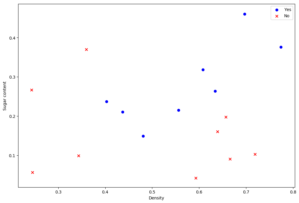
data = pd.read_csv("work/西瓜数据集3.0α.txt")
X = np.array(data[['Density', 'Sugar content']])
y = np.array(data['Good melon']) == '是'
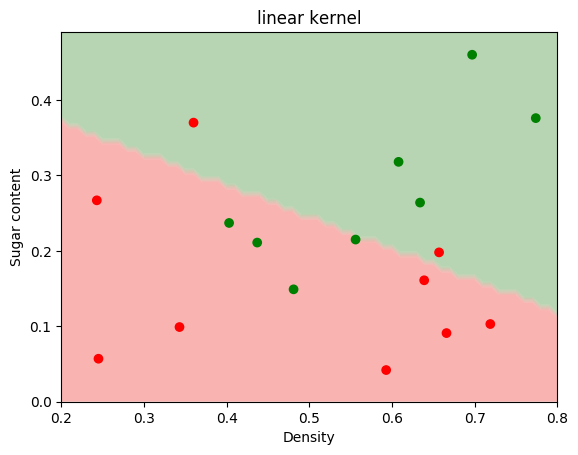
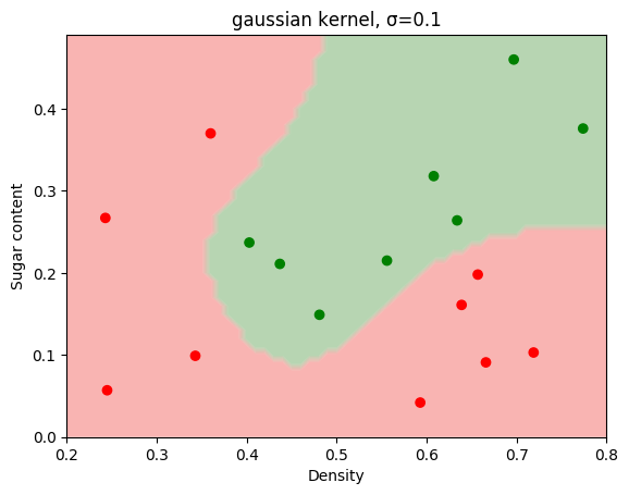
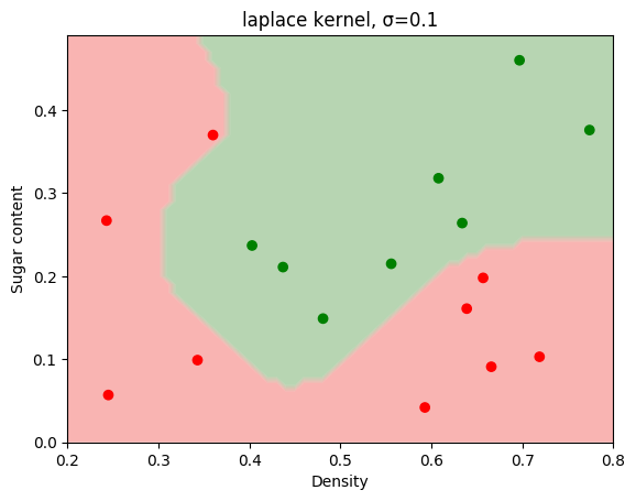
kernels = ['poly', 'gaussian', 'laplace']
titles = ['linear kernel', 'gaussian kernel, σ=0.1', 'laplace kernel, σ=0.1']
for i in range(0, len(kernels)):
model = LogisticRegression(kernel=kernels[i])
model.fit(X, y)
cmap = colors.LinearSegmentedColormap.from_list('watermelon', ['red', 'green'])
xx, yy = np.meshgrid(np.arange(0.2, 0.8, 0.01), np.arange(0.0, 0.5, 0.01))
Z = model.predict(np.c_[xx.ravel(), yy.ravel()])
Z = Z.reshape(xx.shape)
plt.contourf(xx, yy, Z, cmap=cmap, alpha=0.3, antialiased=True)
plt.scatter(X[:, 0], X[:, 1], c=y, cmap=cmap)
plt.xlabel('Density')
plt.ylabel('Sugar content')
plt.title(titles[i])
plt.show()
|