上机实验9:神经网络
任务1:神经元模型
给定数据集X和y
请补全以下代码以实现一个简单的神经元模型(即不包含隐层),并计算模型的参数向量w_vec
待补全代码
1
2
3
4
5
6
7
8
9
10
11
12
13
14
15
16
17
18
19
20
21
22
23
24
25
26
27
28
29
30
31
32
33
34
35
36
37
38
39
40
41
42
43
44
45
46
import numpy as npimport pandas as pdX = np.array([ [0 ,0 ,1 ], [1 ,1 ,1 ], [1 ,0 ,1 ], [0 ,1 ,1 ]]) y = np.array([[0 ,1 ,1 ,0 ]]).T def sigmoid (x, derivative = False ): sigmoid_value =1 / (1 + np.exp(-x)) if derivative == False : return sigmoid_value elif derivative == True : return sigmoid_value * (1 - sigmoid_value) iter_num = 1000 eta = 0.1 num, dim = X.shape w_vec = np.ones((dim, 1 )) for iter in range (iter_num): z_1 = X.dot(w_vec) a_1 = sigmoid(z_1) error = a_1 - y w_vec_delta = X.T.dot(error * sigmoid(z_1, derivative=True )) w_vec = w_vec + eta*w_vec_delta print (w_vec)
[[0.94321144]
 [1.83125284]
 [4.71149329]]
任务2: 感知机
1.感知机是根据输入实例的特征向量x
f (x ) = sign (w ⋅ x + b )
感知机模型对应于输入空间(特征空间)中的分离超平面w ⋅ x + b = 0
2.感知机学习的策略是极小化损失函数:
minw , b L (w , b ) = −∑x i M y i w ⋅ x i b )
损失函数对应于误分类点到分离超平面的总距离。
3.感知机学习算法是基于随机梯度下降法的对损失函数的最优化算法,有原始形式和对偶形式。算法简单且易于实现。原始形式中,首先任意选取一个超平面,然后用梯度下降法不断极小化目标函数。在这个过程中一次随机选取一个误分类点使其梯度下降。
4.当训练数据集线性可分时,感知机学习算法是收敛的。感知机算法在训练数据集上的误分类次数k
$$
k \leqslant\left(\frac{R}{\gamma}\right)^{2}
$$
当训练数据集线性可分时,感知机学习算法存在无穷多个解,其解由于不同的初值或不同的迭代顺序而可能有所不同。
随机梯度下降算法 Stochastic Gradient Descent:
随机抽取一个误分类点使其梯度下降。
w = w + η y i x i
b = b + η y i
当实例点被误分类,即位于分离超平面的错误侧,则调整w b
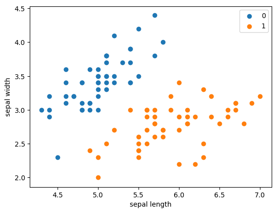
使用iris数据集中两个类别的数据和[sepal length,sepal
width]作为特征,进行感知机分类。
自定义感知机模型,实现iris数据分类;
调用sklearn中Perceptron函数来分类;
验证感知机为什么不能表示异或(选做)。
1.
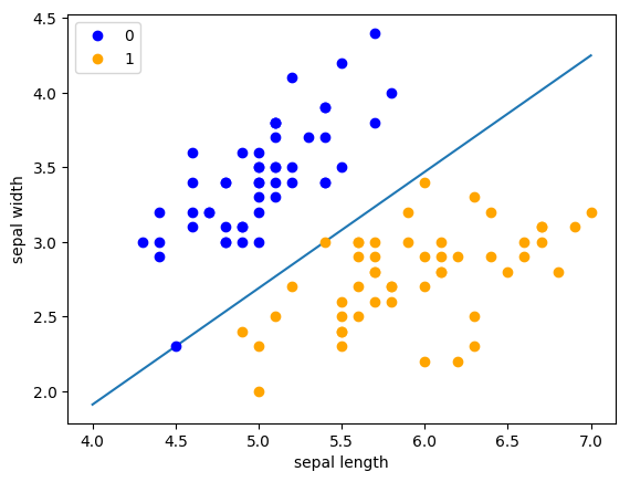
自定义感知机模型,实现iris数据分类
1
2
3
4
5
6
7
8
9
10
11
12
13
14
15
16
17
18
19
20
21
22
23
24
import pandas as pdimport numpy as npfrom sklearn.datasets import load_irisimport matplotlib.pyplot as pltiris = load_iris() df = pd.DataFrame(iris.data, columns=iris.feature_names) df['label' ] = iris.target df.columns = [ 'sepal length' , 'sepal width' , 'petal length' , 'petal width' , 'label' ] df.label.value_counts() data = np.array(df.iloc[:100 , [0 , 1 , -1 ]]) X, y = data[:,:-1 ], data[:,-1 ] y = np.array([1 if i == 1 else -1 for i in y]) plt.scatter(df[:50 ]['sepal length' ], df[:50 ]['sepal width' ], label='0' ) plt.scatter(df[50 :100 ]['sepal length' ], df[50 :100 ]['sepal width' ], label='1' ) plt.xlabel('sepal length' ) plt.ylabel('sepal width' ) plt.legend()
<matplotlib.legend.Legend at 0x7f177628f110>


/opt/conda/envs/python35-paddle120-env/lib/python3.7/site-packages/matplotlib/font_manager.py:1331: UserWarning: findfont: Font family ['sans-serif'] not found. Falling back to DejaVu Sans
  (prop.get_family(), self.defaultFamily[fontext]))
output_6_2
待补全代码
1 2 3 4 5 6 7 8 9 10 11 12 13 14 15 16 17 18 19 20 21 22 23 24 25 26 27 28 29 30 31 class Model : def __init__ (self ): self .w = np.ones(len (data[0 ]) - 1 , dtype=np.float32) self .b = 0 self .l_rate = 0.1 def f (self, x, w, b ): y = np.sign(np.dot(x, w) + b) return y def fit (self, X_train, y_train ): is_wrong = False while not is_wrong: wrong_count = 0 for d in range (len (X_train)): X = X_train[d] y = y_train[d] if y * (np.dot(X, self .w) + self .b) <= 0 : self .w = self .w + self .l_rate * y * X self .b = self .b + self .l_rate * y wrong_count += 1 if wrong_count == 0 : is_wrong = True return 'Perceptron Model!' def score (self ): pass
1 2 3 4 5 6 7 8 9 10 11 12 13 perceptron = Model() perceptron.fit(X, y) x_points = np.linspace(4 , 7 , 10 ) y_ = -(perceptron.w[0 ] * x_points + perceptron.b) / perceptron.w[1 ] plt.plot(x_points, y_) plt.plot(data[:50 , 0 ], data[:50 , 1 ], 'bo' , color='blue' , label='0' ) plt.plot(data[50 :100 , 0 ], data[50 :100 , 1 ], 'bo' , color='orange' , label='1' ) plt.xlabel('sepal length' ) plt.ylabel('sepal width' ) plt.legend()
<matplotlib.legend.Legend at 0x7f1773a0c950>
output_9_1
2.
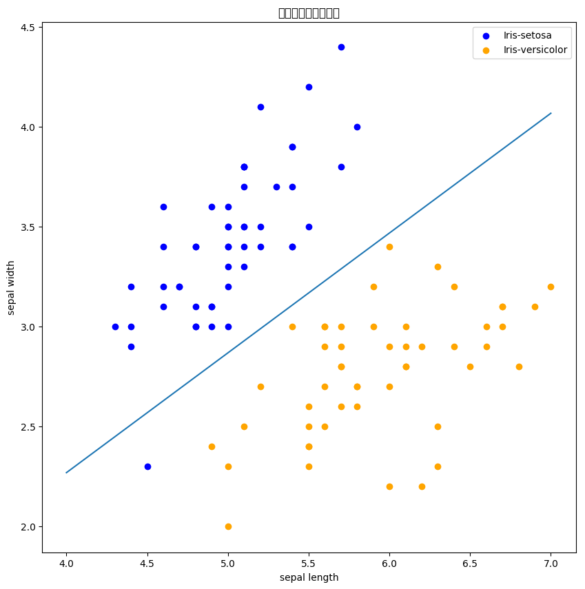
调用sklearn中Perceptron函数来分类
1
2
3
4
5
6
7
8
9
10
11
12
13
14
15
import sklearnfrom sklearn.linear_model import Perceptronclf = Perceptron( max_iter=5000 , eta0=0.05 , shuffle=True ) clf.fit(X, y) print (clf.coef_)print (clf.intercept_)
[[ 1.16  -1.935]]
[-0.25]
1 2 3 4 5 6 7 8 9 10 11 12 13 14 15 16 17 18 19 20 21 22 plt.figure(figsize=(10 ,10 )) plt.rcParams['font.sans-serif' ]=['SimHei' ] plt.rcParams['axes.unicode_minus' ] = False plt.title('鸢尾花线性数据示例' ) plt.scatter(data[:50 , 0 ], data[:50 , 1 ], c='b' , label='Iris-setosa' ,) plt.scatter(data[50 :100 , 0 ], data[50 :100 , 1 ], c='orange' , label='Iris-versicolor' ) x_ponits = np.arange(4 , 8 ) y_ = -(clf.coef_[0 ][0 ]*x_ponits + clf.intercept_)/clf.coef_[0 ][1 ] plt.plot(x_ponits, y_) plt.legend() plt.grid(False ) plt.xlabel('sepal length' ) plt.ylabel('sepal width' ) plt.legend()
<matplotlib.legend.Legend at 0x7f1769a4eb50>
/opt/conda/envs/python35-paddle120-env/lib/python3.7/site-packages/matplotlib/font_manager.py:1331: UserWarning: findfont: Font family ['sans-serif'] not found. Falling back to DejaVu Sans
(prop.get_family(), self.defaultFamily[fontext]))
output_12_2
3.
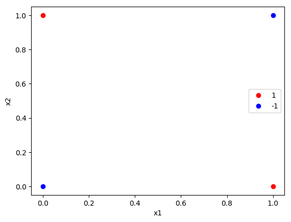
验证感知机为什么不能表示异或(选做)
1 2 3 4 5 6 7 8 9 10 11 12 13 14 15 16 17 18 19 20 21 22 23 24 25 26 27 28 29 30 31 32 33 import numpy as npfrom sklearn.linear_model import Perceptronimport matplotlib.pyplot as pltx=np.array([[1 ,0 ],[0 ,1 ],[0 ,0 ],[1 ,1 ]]) y=np.array([1 , 1 , -1 , -1 ]) plt.plot(x[:2 ,0 ],x[:2 ,1 ],'bo' ,color='red' ,label='1' ) plt.plot(x[2 :4 ,0 ],x[2 :4 ,1 ],'bo' ,color='blue' ,label='-1' ) plt.xlabel('x1' ) plt.ylabel('x2' ) plt.legend() clf = Perceptron( max_iter=1000 , eta0=0.1 , random_state=42 , shuffle=True ) clf.fit(X, y) print ("特征权重 (w):" , clf.coef_)print ("截距 (b):" , clf.intercept_)predictions = clf.predict(X) print ("预测结果:" , predictions)print ("真实标签:" , y)
特征权重 (w): [[0. 0.]]
截距 (b): [0.]
预测结果: [-1 -1 -1 -1]
真实标签: [ 1  1 -1 -1]


/opt/conda/envs/python35-paddle120-env/lib/python3.7/site-packages/matplotlib/font_manager.py:1331: UserWarning: findfont: Font family ['sans-serif'] not found. Falling back to DejaVu Sans
  (prop.get_family(), self.defaultFamily[fontext]))
output_14_2